import opentop as top

actype = "A320"
origin = "EHAM"
destination = "LGAV"

# initial mass as the fraction of maximum takeoff mass
m0 = 0.85 9 🍳 Simple optimal flights
9.1 Quick start
Example code to generate a fuel-optimal flight between two airports. First, we need to set up a few parameters, including origin, destination, actype, and m0 (initial mass).
The initial mass m0 can be the fraction of the maximum take-off mass (between 0 and 1), or it can be the mass in kg (for example, 65000 kg).
In this simple example, we will generate a complete flight using top.CompleteFlight(). We will generate a fuel-optimal flight by setting objective to "fuel" in the trajectory generation function.
optimizer = top.CompleteFlight(actype, origin, destination, m0=m0)

flight = optimizer.trajectory(objective="fuel")
flight.head()| mass | ts | x | y | h | latitude | longitude | altitude | mach | tas | vertical_rate | heading | fuel_cost | grid_cost | fuelflow | |
|---|---|---|---|---|---|---|---|---|---|---|---|---|---|---|---|
| 0 | 66299.999901 | 0.0000 | -652425.011792 | 840651.921719 | 30.480000 | 52.316584 | 4.746242 | 100.0 | 0.300000 | 198.3755 | 2418.0 | 129.5056 | 438.238564 | NaN | 1.872298 |
| 1 | 65856.885789 | 234.0712 | -634430.718537 | 825815.639165 | 2905.430674 | 52.204103 | 5.035375 | 9532.0 | 0.500000 | 319.7176 | 1972.0 | 136.9787 | 347.152728 | NaN | 1.483132 |
| 2 | 65515.244192 | 468.1423 | -608588.389717 | 798123.740055 | 5250.205971 | 51.984433 | 5.459106 | 17225.0 | 0.616216 | 382.7162 | 1472.0 | 136.9787 | 301.376539 | NaN | 1.287565 |
| 3 | 65221.763982 | 702.2135 | -577523.383441 | 764835.369122 | 7000.440553 | 51.718398 | 5.963012 | 22967.0 | 0.704296 | 427.5134 | 1121.0 | 136.9787 | 272.399599 | NaN | 1.163877 |
| 4 | 64956.994546 | 936.2846 | -542727.521179 | 727549.119770 | 8332.820410 | 51.417914 | 6.520452 | 27339.0 | 0.771567 | 459.9134 | 874.0 | 136.9787 | 252.127630 | NaN | 1.077207 |
In the previous table, we have the final fuel-optimal trajectory. Next, we can visualize the altitude, speed, and vertical rate.
import matplotlib
import matplotlib.pyplot as plt

# set up the plot styles
matplotlib.rc("font", size=11)
matplotlib.rc("font", family="Ubuntu")
matplotlib.rc("lines", linewidth=2, markersize=8)
matplotlib.rc("grid", color="darkgray", linestyle=":")


# function to make plot nicer
def format_ax(ax):
    ax.spines["right"].set_visible(False)
    ax.spines["top"].set_visible(False)
    ax.yaxis.set_label_coords(-0.1, 1.05)
    ax.yaxis.label.set_rotation(0)
    ax.yaxis.label.set_ha("left")
    ax.grid()


fig, (ax1, ax2, ax3) = plt.subplots(3, 1, figsize=(5, 4), sharex=True)
ax1.plot(flight.ts, flight.altitude)
ax2.plot(flight.ts, flight.tas)
ax3.plot(flight.ts, flight.vertical_rate)
ax1.set_ylim(0, 40000)
ax2.set_ylim(0, 600)
ax3.set_ylim(-3000, 3000)
ax1.set_ylabel("altitude (ft)")
ax2.set_ylabel("true airspeed (kts)")
ax3.set_ylabel("vertical rate (ft/min)")
ax3.set_xlabel("time(s)")

for ax in (ax1, ax2, ax3):
    format_ax(ax)

plt.tight_layout()
plt.show()
findfont: Font family 'Ubuntu' not found.
findfont: Font family 'Ubuntu' not found.
findfont: Font family 'Ubuntu' not found.
findfont: Font family 'Ubuntu' not found.
findfont: Font family 'Ubuntu' not found.
findfont: Font family 'Ubuntu' not found.
findfont: Font family 'Ubuntu' not found.
findfont: Font family 'Ubuntu' not found.
findfont: Font family 'Ubuntu' not found.
findfont: Font family 'Ubuntu' not found.
findfont: Font family 'Ubuntu' not found.
findfont: Font family 'Ubuntu' not found.
findfont: Font family 'Ubuntu' not found.
findfont: Font family 'Ubuntu' not found.
findfont: Font family 'Ubuntu' not found.
findfont: Font family 'Ubuntu' not found.
findfont: Font family 'Ubuntu' not found.
findfont: Font family 'Ubuntu' not found.
findfont: Font family 'Ubuntu' not found.
findfont: Font family 'Ubuntu' not found.
findfont: Font family 'Ubuntu' not found.
findfont: Font family 'Ubuntu' not found.
findfont: Font family 'Ubuntu' not found.
findfont: Font family 'Ubuntu' not found.
findfont: Font family 'Ubuntu' not found.
findfont: Font family 'Ubuntu' not found.
findfont: Font family 'Ubuntu' not found.
findfont: Font family 'Ubuntu' not found.
findfont: Font family 'Ubuntu' not found.
findfont: Font family 'Ubuntu' not found.
findfont: Font family 'Ubuntu' not found.
findfont: Font family 'Ubuntu' not found.
findfont: Font family 'Ubuntu' not found.
findfont: Font family 'Ubuntu' not found.
findfont: Font family 'Ubuntu' not found.
findfont: Font family 'Ubuntu' not found.
findfont: Font family 'Ubuntu' not found.
findfont: Font family 'Ubuntu' not found.
findfont: Font family 'Ubuntu' not found.
findfont: Font family 'Ubuntu' not found.
findfont: Font family 'Ubuntu' not found.
findfont: Font family 'Ubuntu' not found.
findfont: Font family 'Ubuntu' not found.
findfont: Font family 'Ubuntu' not found.
findfont: Font family 'Ubuntu' not found.
findfont: Font family 'Ubuntu' not found.
findfont: Font family 'Ubuntu' not found.
findfont: Font family 'Ubuntu' not found.
findfont: Font family 'Ubuntu' not found.
findfont: Font family 'Ubuntu' not found.
findfont: Font family 'Ubuntu' not found.
findfont: Font family 'Ubuntu' not found.
findfont: Font family 'Ubuntu' not found.
findfont: Font family 'Ubuntu' not found.
findfont: Font family 'Ubuntu' not found.
findfont: Font family 'Ubuntu' not found.
findfont: Font family 'Ubuntu' not found.
findfont: Font family 'Ubuntu' not found.
findfont: Font family 'Ubuntu' not found.
findfont: Font family 'Ubuntu' not found.
findfont: Font family 'Ubuntu' not found.
findfont: Font family 'Ubuntu' not found.
findfont: Font family 'Ubuntu' not found.
findfont: Font family 'Ubuntu' not found.
findfont: Font family 'Ubuntu' not found.
findfont: Font family 'Ubuntu' not found.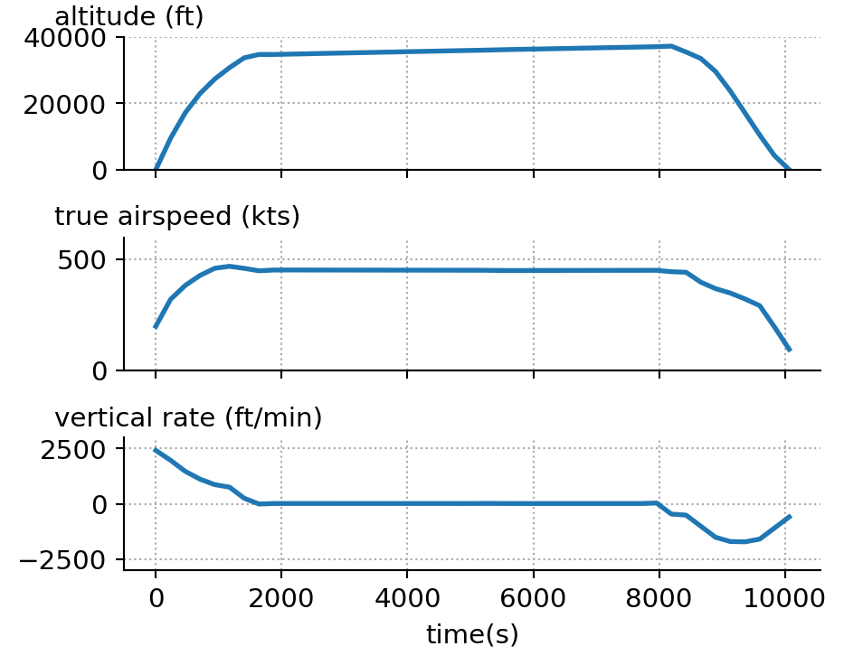
9.2 Other objective functions
Instead of the default objective functions, you can also specify different objective functions as follows:
# cost index, between 0 - 100
flight = optimizer.trajectory(objective="ci:30")
# global warming potential
flight = optimizer.trajectory(objective="gwp100")
# global temperature potential
flight = optimizer.trajectory(objective="gtp100")The final flight object is a pandas DataFrame.
9.3 Different flight phases
Instead of generating a complete flight, we can also generate cruise, climb, and descent flights using top.Cruise, top.Climb, and top.Descent classes.
cruise_flight = top.Cruise(actype, origin, destination, m0=m0).trajectory()
climb_flight = top.Climb(actype, origin, destination, m0=m0).trajectory()
descent_flight = top.Descent(actype, origin, destination, m0=m0).trajectory()There is also a top.MultiPhase optimizer which solves the three phases sequentially as independent problems (climb → cruise → descent), passing each phase’s terminal state as the next phase’s initial state. This is typically more robust than CompleteFlight on longer routes where the full problem is harder to converge:
multiphase_flight = top.MultiPhase(actype, origin, destination, m0=m0).trajectory(
objective="fuel"
)MultiPhase also accepts a per-phase objective as a 3-tuple:
# cost index 60 for climb, 10 for cruise, 20 for descent
multiphase_flight = top.MultiPhase(actype, origin, destination, m0=m0).trajectory(
objective=("ci:60", "ci:10", "ci:20")
)9.4 Choosing a different engine
By default, the optimizer uses the default engine of the aircraft type. Pass engine="..." to use any other engine from the OpenAP prop database:
optimizer = top.CompleteFlight(actype, origin, destination, m0, engine="CFM56-5B4")9.5 Inspecting the result
The DataFrame returned by .trajectory() includes a fuel_cost column (kg of fuel burned per trajectory segment) and a grid_cost column (per-segment grid cost when an interpolant is supplied, otherwise NaN):
flight["fuel_cost"].sum() # total fuel in kgThe optimizer object exposes the solver state after the solve:
optimizer.objective_value # final objective value
optimizer.solver # ca.OptiSol
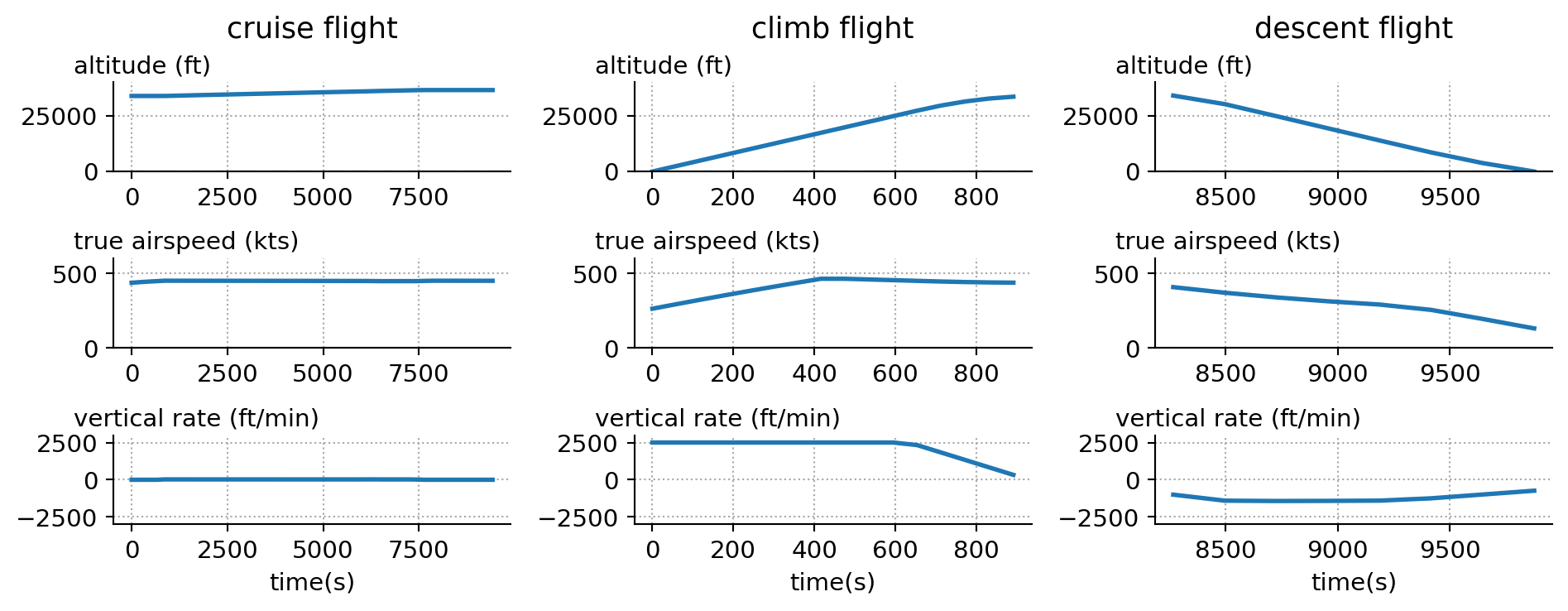
optimizer.solver.stats() # iter_count, success, return_status, ...Let’s visulize these trajectories:
labels = ("cruise flight", "climb flight", "descent flight")
fig, axes = plt.subplots(3, 3, figsize=(10, 4))
for i, flight in enumerate([cruise_flight, climb_flight, descent_flight]):
ax1, ax2, ax3 = axes[:, i]
ax1.plot(flight.ts, flight.altitude)
ax2.plot(flight.ts, flight.tas)
ax3.plot(flight.ts, flight.vertical_rate)
ax1.set_ylabel("altitude (ft)")
ax2.set_ylabel("true airspeed (kts)")
ax3.set_ylabel("vertical rate (ft/min)")
ax1.set_ylim(0, 40000)
ax2.set_ylim(0, 600)
ax3.set_ylim(-3000, 3000)
ax1.set_title(labels[i], pad=20)
ax3.set_xlabel("time(s)")
for ax in axes.flatten():
format_ax(ax)
plt.tight_layout()
plt.show()findfont: Font family 'Ubuntu' not found.
findfont: Font family 'Ubuntu' not found.
findfont: Font family 'Ubuntu' not found.
findfont: Font family 'Ubuntu' not found.
findfont: Font family 'Ubuntu' not found.
findfont: Font family 'Ubuntu' not found.
findfont: Font family 'Ubuntu' not found.
findfont: Font family 'Ubuntu' not found.
findfont: Font family 'Ubuntu' not found.
findfont: Font family 'Ubuntu' not found.
findfont: Font family 'Ubuntu' not found.
findfont: Font family 'Ubuntu' not found.
findfont: Font family 'Ubuntu' not found.
findfont: Font family 'Ubuntu' not found.
findfont: Font family 'Ubuntu' not found.
findfont: Font family 'Ubuntu' not found.
findfont: Font family 'Ubuntu' not found.
findfont: Font family 'Ubuntu' not found.
findfont: Font family 'Ubuntu' not found.
findfont: Font family 'Ubuntu' not found.
findfont: Font family 'Ubuntu' not found.
findfont: Font family 'Ubuntu' not found.
findfont: Font family 'Ubuntu' not found.
findfont: Font family 'Ubuntu' not found.
findfont: Font family 'Ubuntu' not found.
findfont: Font family 'Ubuntu' not found.
findfont: Font family 'Ubuntu' not found.
findfont: Font family 'Ubuntu' not found.
findfont: Font family 'Ubuntu' not found.
findfont: Font family 'Ubuntu' not found.
findfont: Font family 'Ubuntu' not found.
findfont: Font family 'Ubuntu' not found.
findfont: Font family 'Ubuntu' not found.
findfont: Font family 'Ubuntu' not found.
findfont: Font family 'Ubuntu' not found.
findfont: Font family 'Ubuntu' not found.
findfont: Font family 'Ubuntu' not found.
findfont: Font family 'Ubuntu' not found.
findfont: Font family 'Ubuntu' not found.
findfont: Font family 'Ubuntu' not found.
findfont: Font family 'Ubuntu' not found.
findfont: Font family 'Ubuntu' not found.
findfont: Font family 'Ubuntu' not found.
findfont: Font family 'Ubuntu' not found.
findfont: Font family 'Ubuntu' not found.
findfont: Font family 'Ubuntu' not found.
findfont: Font family 'Ubuntu' not found.
findfont: Font family 'Ubuntu' not found.
findfont: Font family 'Ubuntu' not found.
findfont: Font family 'Ubuntu' not found.
findfont: Font family 'Ubuntu' not found.
findfont: Font family 'Ubuntu' not found.
findfont: Font family 'Ubuntu' not found.
findfont: Font family 'Ubuntu' not found.
findfont: Font family 'Ubuntu' not found.
findfont: Font family 'Ubuntu' not found.
findfont: Font family 'Ubuntu' not found.
findfont: Font family 'Ubuntu' not found.
findfont: Font family 'Ubuntu' not found.
findfont: Font family 'Ubuntu' not found.
findfont: Font family 'Ubuntu' not found.
findfont: Font family 'Ubuntu' not found.
findfont: Font family 'Ubuntu' not found.
findfont: Font family 'Ubuntu' not found.
findfont: Font family 'Ubuntu' not found.
findfont: Font family 'Ubuntu' not found.
findfont: Font family 'Ubuntu' not found.
findfont: Font family 'Ubuntu' not found.
findfont: Font family 'Ubuntu' not found.
findfont: Font family 'Ubuntu' not found.
findfont: Font family 'Ubuntu' not found.
findfont: Font family 'Ubuntu' not found.
findfont: Font family 'Ubuntu' not found.
findfont: Font family 'Ubuntu' not found.
findfont: Font family 'Ubuntu' not found.
findfont: Font family 'Ubuntu' not found.
findfont: Font family 'Ubuntu' not found.
findfont: Font family 'Ubuntu' not found.
findfont: Font family 'Ubuntu' not found.
findfont: Font family 'Ubuntu' not found.
findfont: Font family 'Ubuntu' not found.
findfont: Font family 'Ubuntu' not found.
findfont: Font family 'Ubuntu' not found.
findfont: Font family 'Ubuntu' not found.
findfont: Font family 'Ubuntu' not found.
findfont: Font family 'Ubuntu' not found.
findfont: Font family 'Ubuntu' not found.
findfont: Font family 'Ubuntu' not found.
findfont: Font family 'Ubuntu' not found.
findfont: Font family 'Ubuntu' not found.
findfont: Font family 'Ubuntu' not found.
findfont: Font family 'Ubuntu' not found.
findfont: Font family 'Ubuntu' not found.
findfont: Font family 'Ubuntu' not found.
findfont: Font family 'Ubuntu' not found.
findfont: Font family 'Ubuntu' not found.
findfont: Font family 'Ubuntu' not found.
findfont: Font family 'Ubuntu' not found.
findfont: Font family 'Ubuntu' not found.
findfont: Font family 'Ubuntu' not found.
findfont: Font family 'Ubuntu' not found.
findfont: Font family 'Ubuntu' not found.
findfont: Font family 'Ubuntu' not found.
findfont: Font family 'Ubuntu' not found.
findfont: Font family 'Ubuntu' not found.
findfont: Font family 'Ubuntu' not found.
findfont: Font family 'Ubuntu' not found.
findfont: Font family 'Ubuntu' not found.
findfont: Font family 'Ubuntu' not found.
findfont: Font family 'Ubuntu' not found.
findfont: Font family 'Ubuntu' not found.
findfont: Font family 'Ubuntu' not found.
findfont: Font family 'Ubuntu' not found.
findfont: Font family 'Ubuntu' not found.
findfont: Font family 'Ubuntu' not found.
findfont: Font family 'Ubuntu' not found.
findfont: Font family 'Ubuntu' not found.
findfont: Font family 'Ubuntu' not found.
findfont: Font family 'Ubuntu' not found.
findfont: Font family 'Ubuntu' not found.
findfont: Font family 'Ubuntu' not found.
findfont: Font family 'Ubuntu' not found.
findfont: Font family 'Ubuntu' not found.
findfont: Font family 'Ubuntu' not found.
findfont: Font family 'Ubuntu' not found.
findfont: Font family 'Ubuntu' not found.
findfont: Font family 'Ubuntu' not found.
findfont: Font family 'Ubuntu' not found.
findfont: Font family 'Ubuntu' not found.
findfont: Font family 'Ubuntu' not found.
findfont: Font family 'Ubuntu' not found.
findfont: Font family 'Ubuntu' not found.
findfont: Font family 'Ubuntu' not found.
findfont: Font family 'Ubuntu' not found.
findfont: Font family 'Ubuntu' not found.
findfont: Font family 'Ubuntu' not found.
findfont: Font family 'Ubuntu' not found.
findfont: Font family 'Ubuntu' not found.
findfont: Font family 'Ubuntu' not found.