from openap import FuelFlow

# create a fuel flow model for A320
fuelflow = FuelFlow(ac='A320')

# estimate fuel flow during cruise
FF = fuelflow.enroute(mass=60000, tas=230, alt=32000)

# estimate fuel flow at climb, with vertical speed (feet/min)
FF = fuelflow.enroute(mass=60000, tas=200, alt=20000, vs=1000)

# estimate fuel flow at with a given thrust (e.g., derived from drag model)
FF = fuelflow.at_thrust(acthr=50000, alt=30000)

# estimate fuel flow at takeoff
FF = fuelflow.takeoff(tas=100, alt=0, throttle=1)6 🔥 Fuel and Emission
OpenAP provides estimations of fuel consumption and emissions based on actual flight trajectory data. The models are based on the following work:
- ICAO Aircraft Engine Emissions Databank link
- Polynomial models derived from the acropole model
6.1 Accuracy of the fuel model
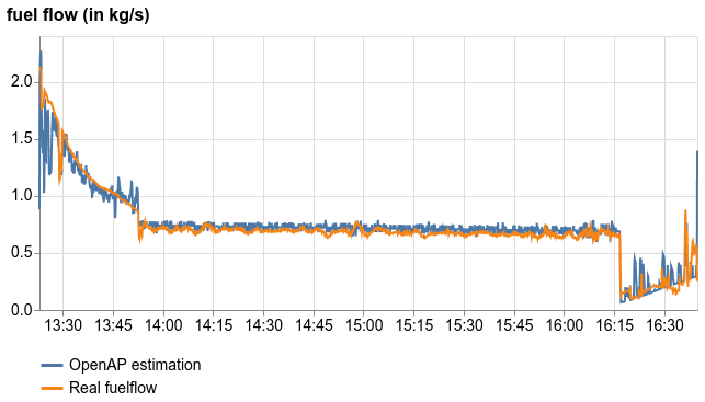
The accuracy of the fuel estimation is greatly improved in the new OpenAP (v2), which is comparable to the BADA 3 fuel model. This is due to the better tuning using data-driven model, acropole, shared by @JarryGabriel.
The acropole model only support a few aircraft types, while the OpenAP extends the model to a wide range of aircraft types based on a customized calibration model based on engine parameters.
The following figure shows the comparison between the fuel flow estimation from OpenAP and the QAR data. In the end of this page, you can find the code snippet to generate this comparison.
6.2 Basic usage of the fuel and emission modules
6.2.1 Compute aircraft fuel flow:
To estimate fuel flow, you need to provide the aircraft type (e.g., ‘A320’) through the openap.FuelFlow object. The fuel flow model is based on: - aircraft’s mass (in kg), - true airspeed (TAS, in kts), - altitude (in ft), - and vertical speed (optional, in ft/min).
6.2.2 Compute aircraft emissions:
The emission model is based on the fuel flow and aircraft’s true airspeed (TAS) and altitude. The input fuel flow is in kg/s The emissions include CO2, H2O, NOx, CO, and HC, with units in g/s.
from openap import FuelFlow, Emission

fuelflow = FuelFlow(ac="A320")
emission = Emission(ac="A320")

TAS = 350
ALT = 30000

FF = fuelflow.enroute(mass=60000, tas=TAS, alt=ALT, vs=0)  # kg/s

CO2 = emission.co2(FF)  # g/s
H2O = emission.h2o(FF)  # g/s
NOx = emission.nox(FF, tas=TAS, alt=ALT)  # g/s
CO = emission.co(FF, tas=TAS, alt=ALT)  # g/s
HC = emission.hc(FF, tas=TAS, alt=ALT)  # g/s
6.3 Estimate fuel and emission from flight data
In the following example, we estimate the fuel consumption for a given flight trajectory data obtained from the OpenSky Network. The sample data can be downloaded from https://github.com/junzis/openap/tree/master/examples.
The following code snippets show how to estimate fuel flow and emissions for this example flight trajectory data.
6.3.1 Data exploration
First, we need to import openap, pandas, and matplotlib libraries.
import pandas as pd
import openap
import matplotlib.pyplot as plt
We also need to define aircraft parameters and import data.
mass_takeoff_assumed = 66300  # kg

fuelflow = openap.FuelFlow("A319")

# Load the data
df = pd.read_csv(
    "data/flight_a319_opensky.csv",
    parse_dates=["timestamp"],
    dtype={"icao24": str},
)

# Calculate seconds between each timestamp
df = df.assign(d_ts=lambda d: d.timestamp.diff().dt.total_seconds().bfill())
Let’s see what are the features in this flight dataframe:
df| timestamp | icao24 | typecode | callsign | origin | destination | latitude | longitude | altitude | groundspeed | track | vertical_rate | d_ts | |
|---|---|---|---|---|---|---|---|---|---|---|---|---|---|
| 0 | 2018-01-02 19:53:00+00:00 | 3946e9 | a319 | AFR91HL | LBG | BMA | 49.085861 | 2.349666 | 8200.0 | 255.0 | 327.804266 | 1920.0 | 60.0 |
| 1 | 2018-01-02 19:54:00+00:00 | 3946e9 | a319 | AFR91HL | LBG | BMA | 49.153427 | 2.310861 | 9475.0 | 290.0 | 9.722018 | 960.0 | 60.0 |
| 2 | 2018-01-02 19:55:00+00:00 | 3946e9 | a319 | AFR91HL | LBG | BMA | 49.233367 | 2.361121 | 9975.0 | 332.0 | 23.243919 | 640.0 | 60.0 |
| 3 | 2018-01-02 19:56:00+00:00 | 3946e9 | a319 | AFR91HL | LBG | BMA | 49.319916 | 2.418471 | 11225.0 | 353.0 | 23.517962 | 2752.0 | 60.0 |
| 4 | 2018-01-02 19:57:00+00:00 | 3946e9 | a319 | AFR91HL | LBG | BMA | 49.411652 | 2.478896 | 14175.0 | 368.0 | 23.566915 | 3584.0 | 60.0 |
| ... | ... | ... | ... | ... | ... | ... | ... | ... | ... | ... | ... | ... | ... |
| 111 | 2018-01-02 21:44:00+00:00 | 3946e9 | a319 | AFR91HL | LBG | BMA | 58.978659 | 17.706646 | 13250.0 | 343.0 | 24.471621 | -1408.0 | 60.0 |
| 112 | 2018-01-02 21:45:00+00:00 | 3946e9 | a319 | AFR91HL | LBG | BMA | 59.062826 | 17.781088 | 11800.0 | 326.0 | 24.443955 | -1344.0 | 60.0 |
| 113 | 2018-01-02 21:46:00+00:00 | 3946e9 | a319 | AFR91HL | LBG | BMA | 59.142609 | 17.852051 | 10400.0 | 307.0 | 24.397686 | -1216.0 | 60.0 |
| 114 | 2018-01-02 21:47:00+00:00 | 3946e9 | a319 | AFR91HL | LBG | BMA | 59.217286 | 17.918701 | 9125.0 | 291.0 | 24.541618 | -1216.0 | 60.0 |
| 115 | 2018-01-02 21:48:00+00:00 | 3946e9 | a319 | AFR91HL | LBG | BMA | 59.289505 | 17.990112 | 8075.0 | 291.0 | 28.500577 | -960.0 | 60.0 |
116 rows × 13 columns
Let’s plot the altitude profile of the flight. I will also make the plots more visually appealing.
from matplotlib import dates

import matplotlib

matplotlib.rc("font", size=11)
matplotlib.rc("font", family="Ubuntu")
matplotlib.rc("lines", linewidth=2, markersize=8)
matplotlib.rc("grid", color="darkgray", linestyle=":")


def format_ax(ax):
    ax.xaxis.set_major_formatter(dates.DateFormatter("%H:%M"))
    ax.spines["right"].set_visible(False)
    ax.spines["top"].set_visible(False)
    ax.yaxis.set_label_coords(-0.1, 1.03)
    ax.yaxis.label.set_rotation(0)
    ax.yaxis.label.set_ha("left")
    ax.grid()


fig, (ax1, ax2, ax3) = plt.subplots(3, 1, figsize=(5, 5), sharex=True)

ax1.plot(df.timestamp, df.altitude)
ax2.plot(df.timestamp, df.groundspeed)
ax3.plot(df.timestamp, df.vertical_rate)

ax1.set_ylabel("altitude (ft)")
ax2.set_ylabel("groundspeed (kts)")
ax3.set_ylabel("vertical rate (ft/min)")

for ax in (ax1, ax2, ax3):
    format_ax(ax)

plt.tight_layout()
plt.show()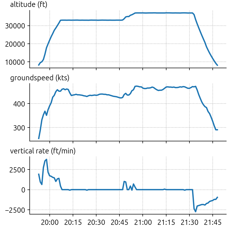
6.3.2 Fuel flow calculation
Next, we iterate over the timestamp to calculate fuel flow and mass during the flight.
mass_current = mass_takeoff_assumed

fuelflow_every_step = []
fuel_every_step = []

for i, row in df.iterrows():
    ff = fuelflow.enroute(
        mass=mass_current,
        tas=row.groundspeed,
        alt=row.altitude,
        vs=row.vertical_rate,
    )
    fuel = ff * row.d_ts
    fuelflow_every_step.append(ff)
    fuel_every_step.append(ff * row.d_ts)
    mass_current -= fuel

df = df.assign(fuel_flow=fuelflow_every_step, fuel=fuel_every_step)
Then, we can visualize the fuel flow during the flight.
plt.figure(figsize=(7, 2))
plt.plot(df.timestamp, df.fuel_flow, color="tab:red")
plt.ylabel("fuel flow (kg/s)")
format_ax(plt.gca())
plt.show()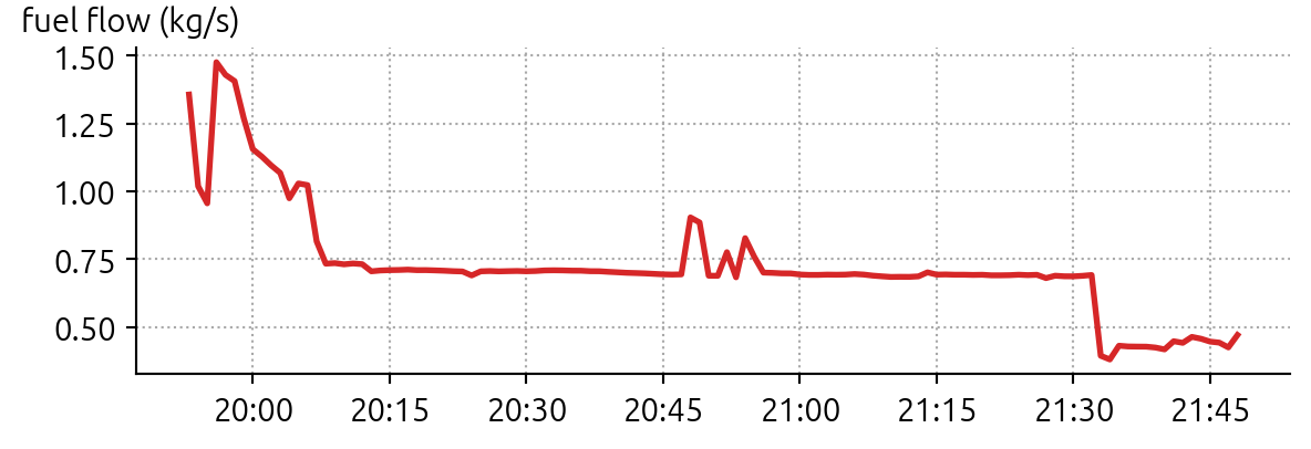
With the new dataframe, we can calculate total fuel consumption by summing the fuel consumption at overall time steps:
total_fuel = df.fuel.sum().astype(int)
print(f"Total fuel: {total_fuel} kg")
Total fuel: 3841 kg6.3.3 Emission calculation
The emission calculations are based on the fuel consumption using the openap.Emission class.
We can calculate the emissions for the entire flight and append them as new columns to the dataframe as follows:
emission = openap.Emission(ac="A319")

df = df.assign(
    co2_flow=lambda d: emission.co2(d.fuel_flow),
    h2o_flow=lambda d: emission.h2o(d.fuel_flow),
    soot_flow=lambda d: emission.soot(d.fuel_flow),
    sox_flow=lambda d: emission.sox(d.fuel_flow),
    nox_flow=lambda d: emission.nox(d.fuel_flow, tas=d.groundspeed, alt=d.altitude),
    co_flow=lambda d: emission.co(d.fuel_flow, tas=d.groundspeed, alt=d.altitude),
    hc_flow=lambda d: emission.hc(d.fuel_flow, tas=d.groundspeed, alt=d.altitude),
)
Let’s visualize the emission flows:
fig, axes = plt.subplots(7, 1, figsize=(5, 7), sharex=True)

axes = axes.flatten()

labels = dict(
    co2_flow="CO2 (g/s)",
    h2o_flow="H2O (g/s)",
    soot_flow="Soot (g/s)",
    sox_flow="SOx (g/s)",
    nox_flow="NOx (g/s)",
    co_flow="CO (g/s)",
    hc_flow="HC (g/s)",
)

for i, (k, v) in enumerate(labels.items()):
    axes[i].plot(df.timestamp, df[k], color="tab:brown")
    axes[i].set_ylabel(v)
    format_ax(axes[i])


plt.tight_layout()
plt.show()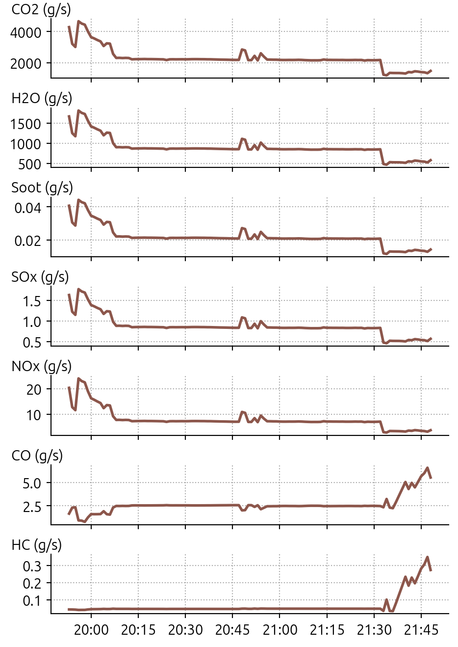
Note that CO2, H2O, Soot, and SOx are linear correlated to the fuel flow, following the coefficients from the paper Global Mortality Attributable to Aircraft Cruise Emissions.
6.3.4 Final data
The emissions at each time step are also calculated as follows. Note that we divide values by 1000 to obtain the emissions in kg.
df = df.eval(
    """
    co2 = co2_flow * d_ts / 1000
    h2o = h2o_flow * d_ts / 1000
    soot = soot_flow * d_ts / 1000
    sox = sox_flow * d_ts / 1000
    nox = nox_flow * d_ts / 1000
    co = co_flow * d_ts / 1000
    hc = hc_flow * d_ts / 1000
    """
)
We can take a look at the final data with fuel flow and emissions columns.
df[["timestamp", "fuel", "co2", "h2o", "soot", "sox", "nox", "co", "hc"]].round(4)| timestamp | fuel | co2 | h2o | soot | sox | nox | co | hc | |
|---|---|---|---|---|---|---|---|---|---|
| 0 | 2018-01-02 19:53:00+00:00 | 84.5375 | 267.1385 | 103.9811 | 0.0025 | 0.1014 | 1.3049 | 0.0892 | 0.0026 |
| 1 | 2018-01-02 19:54:00+00:00 | 59.4300 | 187.7989 | 73.0989 | 0.0018 | 0.0713 | 0.7334 | 0.1397 | 0.0026 |
| 2 | 2018-01-02 19:55:00+00:00 | 54.0898 | 170.9238 | 66.5305 | 0.0016 | 0.0649 | 0.6335 | 0.1421 | 0.0026 |
| 3 | 2018-01-02 19:56:00+00:00 | 91.0999 | 287.8755 | 112.0528 | 0.0027 | 0.1093 | 1.5188 | 0.0434 | 0.0024 |
| 4 | 2018-01-02 19:57:00+00:00 | 88.7208 | 280.3577 | 109.1266 | 0.0027 | 0.1065 | 1.4676 | 0.0391 | 0.0024 |
| ... | ... | ... | ... | ... | ... | ... | ... | ... | ... |
| 111 | 2018-01-02 21:44:00+00:00 | 6.7503 | 21.3311 | 8.3029 | 0.0002 | 0.0081 | 0.0284 | 0.2678 | 0.0160 |
| 112 | 2018-01-02 21:45:00+00:00 | 5.5660 | 17.5885 | 6.8462 | 0.0002 | 0.0067 | 0.0236 | 0.2156 | 0.0129 |
| 113 | 2018-01-02 21:46:00+00:00 | 5.1859 | 16.3875 | 6.3787 | 0.0002 | 0.0062 | 0.0221 | 0.1962 | 0.0117 |
| 114 | 2018-01-02 21:47:00+00:00 | 3.2038 | 10.1240 | 3.9407 | 0.0001 | 0.0038 | 0.0137 | 0.1187 | 0.0071 |
| 115 | 2018-01-02 21:48:00+00:00 | 8.4690 | 26.7619 | 10.4168 | 0.0003 | 0.0102 | 0.0364 | 0.3089 | 0.0185 |
116 rows × 9 columns
Finally, we can obtain the total fuel consumption and emissions for the entire flight (unit in kg).
df[["fuel", "co2", "h2o", "soot", "sox", "nox", "co", "hc"]].sum().round(2)fuel 3841.92
co2 12140.48
h2o 4725.57
soot 0.12
sox 4.61
nox 39.18
co 17.28
hc 0.43
dtype: float646.4 QAR data comparison
The following code snippet shows how to compare the fuel flow estimation from OpenAP with the QAR data. This QAR data is an example flight from traffic library.
fuelflow = openap.FuelFlow(ac="A320")

# Load the data
df = pd.read_csv("data/flight_a320_qar.csv", parse_dates=["timestamp"])

ff_estimate = fuelflow.enroute(
    mass=df.weight, tas=df.TAS, alt=df.altitude, vs=df.vertical_rate
)

diff = abs(ff_estimate.sum() - df.fuelflow.sum()) / df.fuelflow.sum() * 100

plt.figure(figsize=(7, 3))
plt.plot(df.timestamp, df.fuelflow, lw=1, label="QAR")
plt.plot(df.timestamp, ff_estimate, lw=1, label="OpenAP")
plt.ylabel("fuel flow (kg/s)")
plt.legend()
plt.show()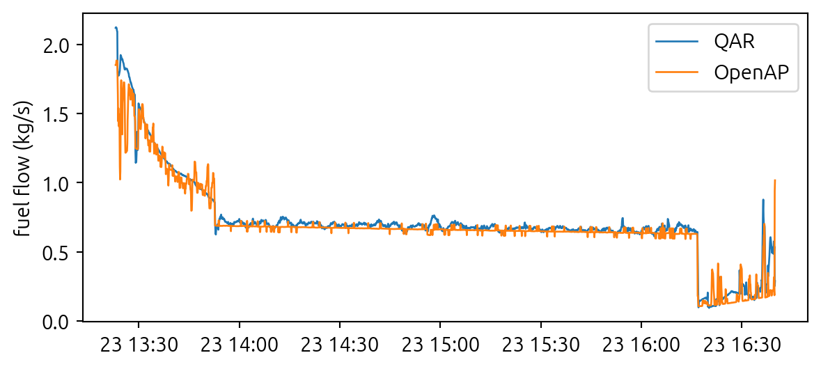
The difference between the estimated fuel flow and the QAR data is 4.29%.